If you are working in an excel spreadsheet there may be times when you are looking at a large area of data and you may need to keep areas of the worksheet visible when you are scrolling to make managing your data easier through simplistic visualisation.
You can do this by using the Freeze Frame feature in Excel. By doing this you can freeze rows along the top of the worksheet and columns to the left. This will mean that if you have important information along the top row and or the left hand column, you can keep it all in view when you are scrolling through all the data. Using the Freeze Frame will allow you to freeze more than one row or column at a time, but please note that you cannot freeze rows or columns in the middle of a worksheet.
-
To freeze rows you select the row beneath the ones that you want to be able to see, so if you wanted to freeze the top two rows, it would mean selecting the row directly under them.
-
With columns, you select the row directly to the right of the rows that you want to remain visible.
-
If you want to freeze both rows and columns, you need to select the cell to the right of the column and directly below the row that you want to freeze, For example if you wanted to freeze column A and row 1, you would click on cell B2.
-
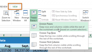
Next, on the ribbon click the View tab, then click the Window group and then Freeze Pane. Thiswill give you the options of,
-
Freeze Panes, which will freeze both the selected rows and columns together, or gives you the option of freezing more than one row or column.
-
Freeze Top Row will just freeze the top row.
-
Freeze First Column will just freeze the first column on the left.

To unfreeze the panes just go back on to the ribbon, to the Freeze pane panel and click Unfreeze Pane.

